
Before we can go any further in our study of personality models, I must explain some things about numbers. In working with personality models, I kept running into stupid mathematical problems that caused me endless headaches. I will not explain all those problems; they’re not fun. Besides, the problem is well-demonstrated in my Lecture #2 which you can see in this video at 11:00: https://www.youtube.com/watch?v=l87BcwMMP6U&t=2s
Instead, I’ll just tell you the solutions I came up with. If you have an endless supply of aspirin, I invite you to reject my number system and explore the delights of conventional mathematical approaches to personality modelling. After all, artists are expected to suffer, right?
As explained in the video above, my solution involves “Bounded Numbers”, which cool people call “BNumbers”. BNumbers have four important properties:
1. The distribution of values of personality traits in the general population is a bell curve.
(Technical note for mathematical nitpickers: it is not a Gaussian curve and the tails don’t extend out to infinity.)
2. The number system has absolute upper and lower limits that can never be passed.
3. Those limits are -1 and +1.
4. The BNumber value 0.0 represents the middle, the average, the normal, the everyday value for most people.
Now, if we were to built a histogram of all the people in the world, we’d expect the distribution of those people to fall along a bell curve, like this:
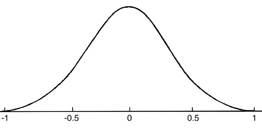
In other words, most people would be around the middle of the bell curve. A few would be at the lower end, and a few would be at the upper end. This explains why I use double labels for my personality traits. Calling it ‘Good’ would imply a one-sided distribution, but calling it ‘Bad_Good’ fits better with the idea of the bell curve. The lower end of the bell curve represents bad people, and the upper end represents good people. In the same way, ‘Faithless_Honest’ describes both ends of the bell curve, as does ‘Timid_Dominant’. I strongly encourage you to follow this protocol in labeling whatever personality traits you create for your personality models; it makes it much easier to recognize the negative and the positive sides of any trait. By the way, the protocol has the negative side coming before the positive side. It’s not ‘Good_Bad’, it’s ‘Bad_Good’.
To help you explore the properties of BNumbers, I provide a spreadsheet that you can use to try them out. There are two versions: Numbers (for Mac) and Excel (for Windows)
Let’s take a tour of the spreadsheet. Most of its elements are easy to figure out, but I’ll be explicit about them here. I have already filled in the first 41 rows for you with a sample set that illustrates the properties of BNumber operators.
Column B: x
This is the first input value used in all the BNumber operators to the right. The column is shaded in cyan to denote the fact that you type input numbers here. Be sure that you enter ONLY numbers between -1.0 and +1.0. I’m too lazy to put safety barriers in here for you.
Column C: y
This is the second input number used in all the BNumber operators to the right. The same restrictions apply.
Column D: Inverse(x)
This is a BNumber operator that transforms a BNumber to a real number. BNumber addition and subtraction convert the BNumbers to real numbers, add or subtract them, then convert the result back to a BNumber. This is how the BNumber system guarantees that your numbers stay within reasonable bounds.
Column E: Inverse(y)
Same as above for y.
Column F: WS+
This is just an intermediate value that shows you the internal details of BSum: it shows the sum of the two real numbers. To get BSum (Column G), we just convert this value to a BNumber.
Column G: BSum
The BSum of x and y.
Column H: WS-
Same as Column F, except for subtraction.
Column I: BDifference
Bounded subtraction of y from x.
Column J: Weight
This is the third input value for the Blend operator, the weight for the shift from x to y.
Column K: uWeight
This is another internal calculation result, this time for the Blend operator.
Column L: Blend(x, y, BWeight)
This is the all-important Blend operator, which you’ll be using heavily. It is explained in Lecture #2 starting at 11:50
Column M: UNumberToBNumber
Occasionally, you might need to use a BNumber that you need to be always positive. In other words, this is a BNumber that has only half the range of a normal BNumber. Instead of running from -1 to +1, as a normal BNumber does, you need a number that runs from 0 to +1. This is not a common problem, but every now and then you really need such a number, and you need to convert a regular BNumber into this “UNumber”. This column converts the BNumber in x to a UNumber. We also have the opposite operator, UNumberToBNumber, but I didn’t bother including it in the spreadsheet. I emphasize that this is not a common issue.
Columns N and O
These columns are used to calculate the slope of the BSum and BDifference operators, which is only of educational value. You can look at the graphs below the spreadsheet to see the slopes, which might be of some value if you like to think in terms of slopes. This is really for math geeks only.
Exercises
Play around with the input values in the spreadsheets. For example, while the x-values increase regularly from -1 to +1, the y-values are constant. Try putting different constant values into the y-column to see how it changes the results. Or try putting variations into the y-values. Also play around with the weighting values in column J.
You might also look at the equations used for the Blend operator. They’re a bit tricky to figure out.
For you math geeks:
I’ve never been quite satisfied with the mathematical structure of the transform from real numbers to BNumbers. The problem is best illustrated in the slope curves for BSum and BDifference in the spreadsheets. Those peaks in the slope graphs make me squirm; I’m uncomfortable with functions that have high localized first and second derivatives; such functions generally do not correspond well to the real world. This bothers me because it means that tiny changes have huge effects with bounded numbers near zero, and almost no effect with bounded numbers near ±1. This is, of course, the basic specification, but my gut tells me that that changes near zero are too large.
The basic transform I use for converting a positive real number into a bounded number is this:
bounded = 1 - (1 / (1 + real number))
This can be generalized to:
bounded = 1 - (a / (a + real number))
If you experiment with different values of a, you’ll find a number of interesting variations in the behavior of the transforms and the resulting slopes of BSum and BDifference. Higher values of a do not change the slope near 0. Interestingly, changes in a do not appear to affect the Blend operator, which is the more commonly used operator. I therefore think that a completely different transform would do a better job. Fifty years ago I could have reached into my mathematical toolkit and cobbled together a better function, but just now I don’t see it. Perhaps further thought will turn on a light bulb somewhere in my mind.
No, we cannot use the equation for the normal distribution; it does not go to zero at ±1. I suppose that we could use such a distribution with standard deviation = 0.3 and a brute force boolean cutoff to zero at 0.9999; only about 0.01% of the area under the curve would be lost this way.
Or we could use the proper normal distribution, but here’s the equation we’d be using:
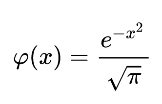
This really isn’t that hard to use, but it would require a lot of additional effort dealing with the extreme values. In general, increments to a value would be calculated from the inverse of probability value of the normal distribution. I think that, for now, we can live with the simplistic BNumber system.
