
Things have been going along rather smoothly: I’ve been adding more background material, tuning the simulation, adding a home page with seven levels of play, and so forth. However, this design diary is prompted by my decision to throw away my resource supply equations and replace them with something entirely new. I was prompted to do this when I began testing the biased versions of the simulation (industry-biased and green-biased). I discovered, to my chagrin, that the industry-biased version went ballistic very quickly, so I had to revise the coefficients. After careful examination of the resource supply formulae, I decided that they were inadequate. Instead, I resolved to implement a sigmoid function, which looks roughly like this:
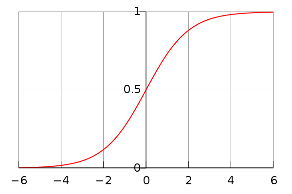
This function is expressed with the formula y(x) = 1 / ( 1 + e**-x). For my purposes, I need add only three coefficients. The first represents the value of the asymptote. In the original formula, that asymptote is 1, but I need it to equal the absolute maximum amount of resource that could be obtained at any price. I shall label this coefficient Smax. For solar photovoltaic energy, for example, its value would be the amount of electricity we could generate if we covered the planet with solar cells (in practice, I think it best to use a smaller value representing something like reality). The second coefficient is more difficult to understand; it sets the horizontal scale and might best be called “Price Sensitivity”, PS. This means that our formula looks like this:
Supply of resource(price) = Smax / (1 + e**-(PS*price)
[You might be wondering why I don’t simply use the Hubbert Curve for this work. As it happens, I *am* using the Hubbert Curve; the curve above represents the integral of the Hubbert Curve, which displays the annual production of a resource, where I am interested in the cumulative production of a resource. Moreover, the Hubbert Curve makes assumptions about constant prices and technology that I do not wish to apply.]
Thus, PS serves to stretch or squeeze the horizontal axis. There remains a problem with this formula: it yields a value of Smax/2 when price = 0. This is wrong; when price = 0, supply should equal zero. I examined a number of solutions to this. None of them produced satisfactory results: anything that shifted the curve so that the zero at negative infinity corresponded to price = 0 also distorted the curve in an unacceptable fashion. Besides, there’s a much simpler kluge: shift the horizontal axis additively, like this:
Supply of resource(price) = Smax / (1 + e**-((PS*price)-offset)
Here, offset is the amount by which the curve is shifted rightwards. This is a mathematically incorrect solution, because it implies non-zero production at negative prices (“How much will you pay me to take that oil off your hands?”) Nevertheless, at no point in this simulation will we encounter negative energy prices, so the problem will never arise. So, how do we calculate the values of Smax, PS, and offset?
Smax is the simplest to figure: it’s the maximum amount of resource we could obtain if money were no object. It’s the amount of hydroelectricity we could get if we damned every river, creek, and stream on the planet. It’s the amount of oil we could get if we pumped every last drop of oil out of the ground. There is a bit of a problem here: nobody really knows the absolute total amount of oil in the ground. We have all sorts of ways of estimating it, but all those estimates are based on the amount of money we’re willing to spend to get it out of the ground. For example, there’s lots of shale oil to recover -- if the price is higher than $120/bbl. Below that price, there’s almost nothing. So, how do I extrapolate from the current estimates to the absolute maximum? There’s no reliable means for doing so, which means that I’m just going to have to guess. And it turns out that by simply doubling the current maximum estimates, I get a solution that also makes the rest of the calculation a bit easier. So that will be my value of Smax: twice the current estimate of highest estimate of recoverable reserves.
This means that the inflection point is the point at which the supply is equal to half of Smax. This is what I estimate to be the maximum recoverable reserves of that resource. I believe that this is actually a big larger than that: I think that “maximum recoverable reserves” represents the amount of reserves at a price somewhat higher than the current price. I could do a lot of research on this question, but I’m too lazy; I shall instead assign a price to that level of reserves. This price will also denote the inflection point in the sigmoid curve. This then gives me a new relationship to use for determining the coefficients of the formula:
Supply of resource(inflection price) = Smax / (1 + e**-((PS*[inflection price])-offset) = Smax / 2
==> e**-((PS*[inflection price])-offset) = 1
==> PS*[inflection price]) = offset
Now I need add only one other consideration: the supply at the current price of $30 billion per exajoule:
Supply of resource($30 billion) = Smax / (1 + e**-((PS*[$30 billion])-offset)
But what is the current supply of the resource? Let’s take oil, for example. Currently we use about 175 exajoules of the stuff every year. Is the supply then 175 exajoules? No, that represents the lower limit of the supply at a price of $30 billion / exajoule.
This is a serious problem, so I went back and did some research. Remember, the simulation need only run for 30 years, during which time we will not exhaust the supply of any of our fossil fuels. The prices will rise, to be sure, but they won’t soar into the stratosphere. So perhaps I don’t need the full sigmoid function. Let’s take the case of oil, for example. My guess is that the overall supply curve looks something like this:
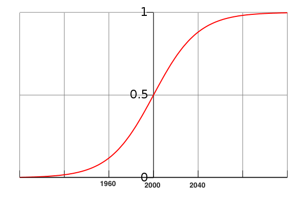
If this is a decent approximation of the reality, then consider that the game runs only from 2012 to 2042; during that period the supply versus price curve is pretty close to linear. We know that the coal curve is even more stretched out, and the natural gas curve might — MIGHT — be more stretched out if the recent discoveries of shale gas prove to be representative of other fields.
This would mean that I’d have a much simpler supply/price curve: each fossil fuel would have a relationship something like this:
Total Supply (price) = a * Price
where a is the controlling coefficient. In other words, if the price doubles, the supply doubles. Inasmuch as I don’t expect the price of energy in this simulation to even double, I think this is a safe approximation. So now the only problem is to determine the value of a for each of the various energy sources. That’s easily obtained: divide the current price by the cumulative amount of the resource that has been consumed. That information is easily enough obtained. First, all energy sources right now can be assumed to be priced at $30 billion per exajoule; this is a little unfair to electric-only sources and a too generous to coal. But I think this simplification is acceptable. Here then are some results:
Cumulative coal consumption: 10,000 exaJoules ==> a = 333
Cumulative oil consumption is about the same as total coal consumption (coal got the early start but oil became much bigger than coal in the second half of the 20th century. Thus, oil gets the same value of a as coal. This may seem strange but remember, we’re only concerned with the next thirty years.
Cumulative natural gas consumption: 7800 exaJoules ==> a = 260
Cumulative nuclear energy consumption: 1080 exaJoules ==> a = 36
Cumulative hydro energy consumption: 700 exaJoules ==> a = 23
Cumulative geothermal energy consumption: 4 exaJoules ==> a = 0.13
Cumulative solar photovoltaic consumption: 0.5 exaJoules ==> a = 0.016
Cumulative wind energy consumption: 10 exaJoules ==> a = 0.33
I’m going to plug these numbers into the simulation and see how it runs.