
I am redesigning Balance of the Planet to work in Javascript so that people all over the web can use it. I am not keeping detailed design diaries because my usage data indicates that not many people read my design diaries. But I am today tackling a particularly difficult problem and I need to talk it out in order to make sense of it, so I might as well make it public. Besides, this is a particularly interesting problem and those few who read it might gain some useful insights.
Here’s the problem: how do I calculate the price of an energy source, based on its particular supply characteristics?That price is, of course, affected by all the other prices, so this will require a convergent algorithm. Complicating matters is the fact that the supply of any energy source changes with the price. For example, hydroelectric energy at very low levels of usage is quite cheap. It’s cheap to slap a dam on a perfectly sited river with a big height differential and lots of water flow. Hence, the first exajoules we get out of hydro are cheap. But if we want more hydro exajoules, we’ll have to build dams on smaller rivers with lower height differentials.
We start with the total demand for energy, then set the price of energy at 0 and step through each of the sources of energy, allocating energy from that source to meet demand in the amount (E($) + E($+1))/2, where E($) is the amount of energy the the source can supply at the price $. We continue this process through each of the energy sources, then increment the price and repeat until the demand for energy is satisfied.
A major flaw in this process is that energy is not demanded smoothly over the course of the year. This is especially important with electricity, whose load demand varies diurnally. The solution to this flaw is so complicated that I conclude that I must overlook it.
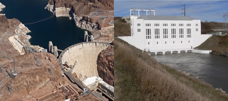
Another flaw arises from the fact that some sources of energy provide small amounts of energy for almost nothing. Hoover Dam, shown above, provides us with electricity at very low cost, but if demand were low enough, would we meet all of our energy demand with electricity from Hoover Dam and throw away everything else? Well, no, so the algorithm I have described will produce absurd results at extremely low levels of demand. I think, however, that such a situation is so unlikely that I needn’t concern myself with it.
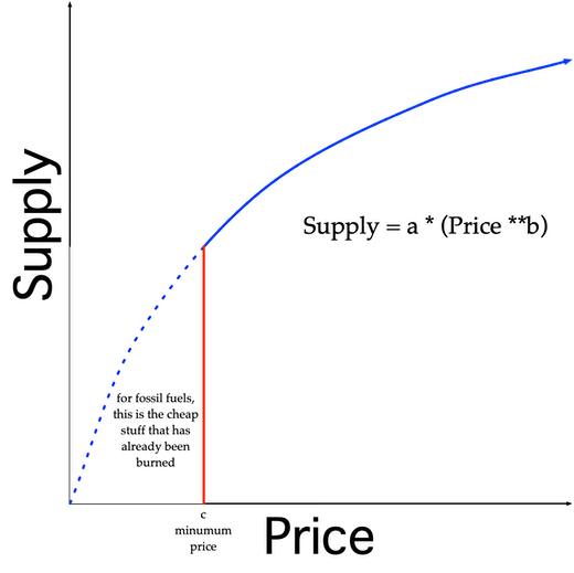
Here’s a graph showing the basic relationship between supply and price. It’s easiest to understand if you apply my earlier discussion of hydro. Sources like Hoover Dam provide lots of cheap energy, but if we want a larger supply of energy, we’ll have to build dams like the one on the right that don’t provide anywhere near as much energy for the cost of operation. If we want more coal, we’ll have to dig deeper. If we want more wind energy, we’ll have to put turbines in less windy places.
The algorithm
For this relationship I use the algorithm:
IF ((Price > c) | (Source is renewable)
Supply = a * (Price**b)
ELSE
Supply = 0
How do I determine the values of a, b, and c? Fortunately, the value of c is simply the lowest current price of the fossil fuel. But determining a and b are tricky business. Renewables and nonrenewables must be handled with entirely different algorithms. Some professors at The Pennsylvania State University have come up with a nice model for oil supplies, which is easily modified to address coal and natural gas. Here’s the basic diagram:
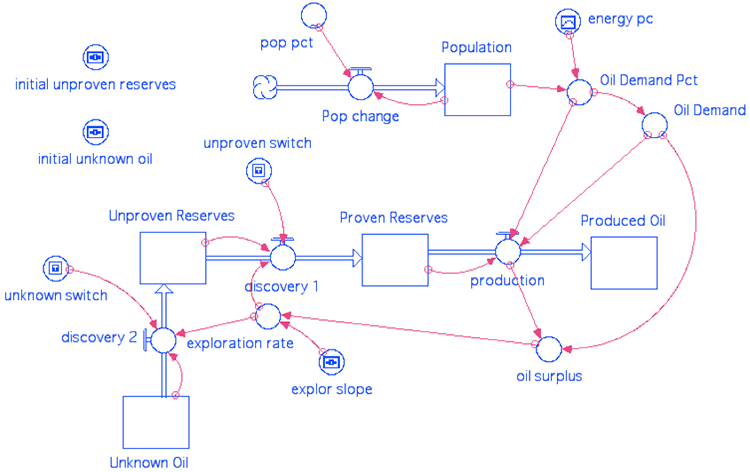
I won’t use their model, because I was unable to find the underlying code. Moreover, my thinking places primary emphasis on economic factors, not technical factors. This is not true when we consider the full range of supply, but I believe that it handes the mid-range of supply where the real world will be working through this century.
Oil resources are characterized by three curves, representing "economically recoverable" reserves (what we can recover at current prices), "technically recoverable" reserves (what we can recover with currently available technology), and "in-place reserves" (the total amount of oil actually in the ground). They also use “proven”, “probable”, and “possible”.
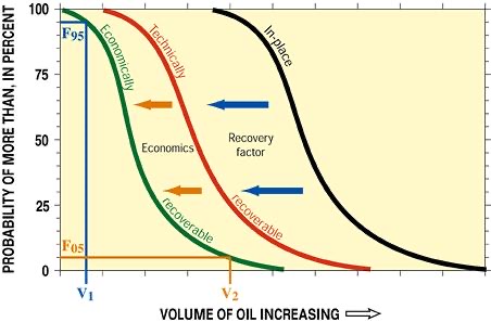
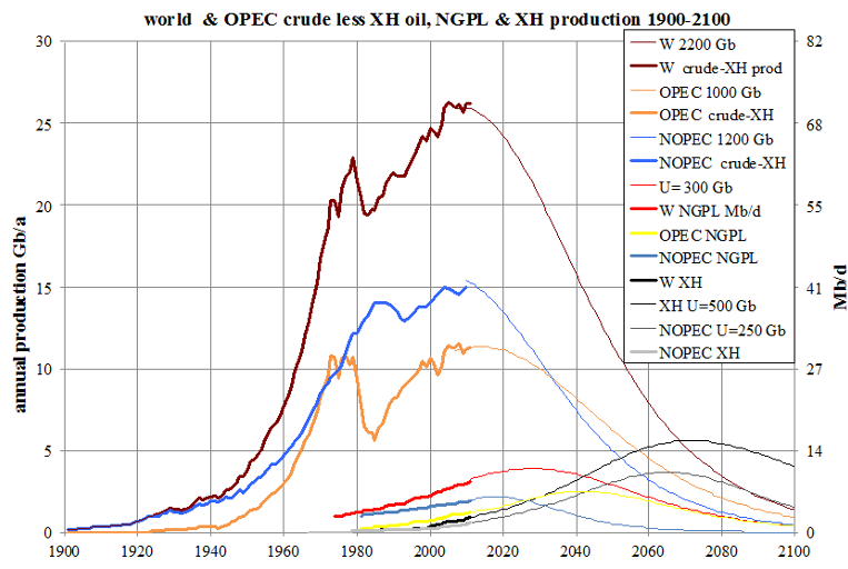
Note that, as the price of oil increases, the green curve moves to the right. Indeed, at the highest levels of consideration, technology improves with the price (the development of fracking providing an excellent example), shifting the red curve to the right. Therefore, I condense the ideas behind this graph down to the simpler graph I present above. To obtain the coefficients used in my graph, I must combine the data from these graphs of actual production of oil and the actual price of oil:
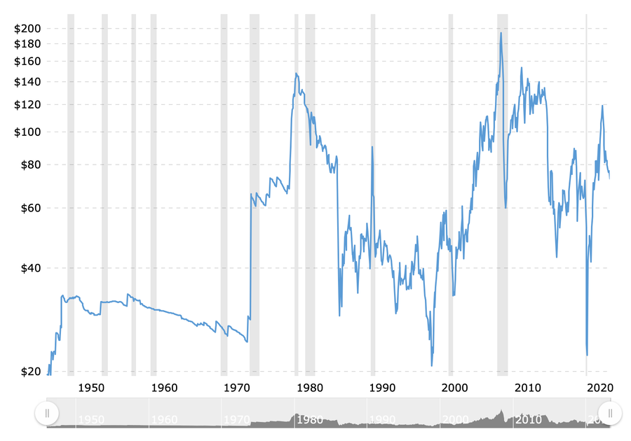
The upper graph is easy to deal with, but the lower graph is a mess, reflecting the development of new technologies and the discovery of new oilfields. Adding to the headaches is the fact that the lower graph is logarithmic (at least it is already inflation-adjusted). Here’s where brutal simplification comes in: I’ll draw a straight line through it, like so:
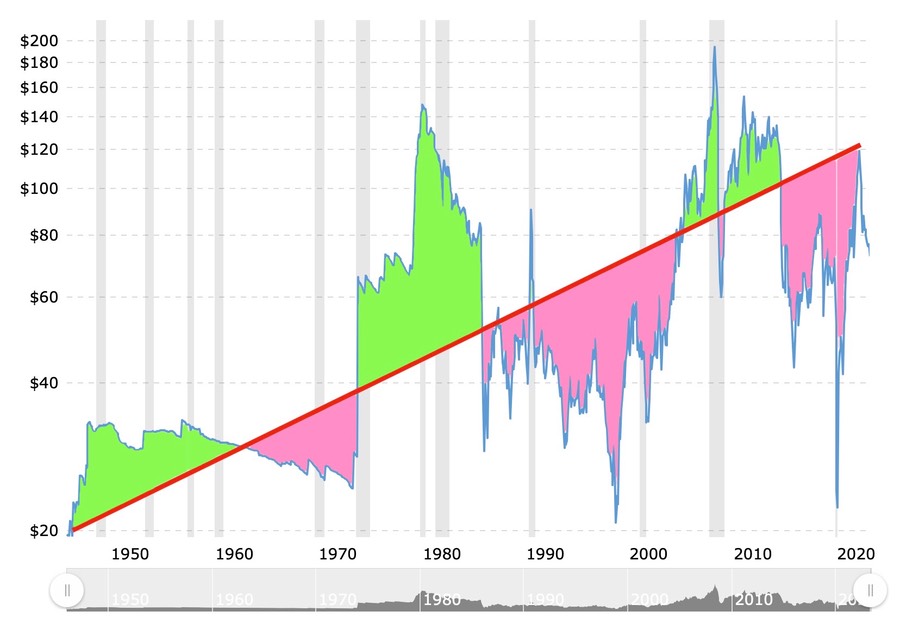
(By the way, here’s my rule of thumb for eyeballing a straight line through a messy graph: try to visually balance the green area against the pink area.) The equation for this line is:
Price = $20 + $95 * (Year - 1945)/75
Remember, this is using a logarithmic scale, so I might want to transform the equation to linearly reflect prices, but I’m too lazy to do that just yet, nor do I see a pressing need to do so.
Next, we must determine the equation for the production figures shown above. This is a bell curve, which is most commonly represented by the equation for what is called the “Gaussian distribution”:
Believe it or not, this can actually be done with this data, because 𝝈 is just the standard deviation of the bell curve, easily calculated directly, and 𝝁 is just the mean of the curve, which is directly observable as the year 2010. I did some quickie calculations and come up with a value for 𝝈 of 32 years. Hence:
Supply = 1/(32*SQRT(2π))*e**(-(1/2)*(year-2010)/32)**2)
Urk! Now I must somehow combine the simple price equation with the horrible supply equation. To do this, I invert the price equation to solve for Year:
Year = (Price - $20)/$95*75 + 1945
Substituting this into the messy Gaussian equation:
Supply = 1/(32*SQRT(2π))*e**(-(1/2)*((Price - $20)/$95*75 + 1945-2010)/32)**2)
Gee, that wasn’t so hard, was it? {evil snigger}. We can at least simplify it somewhat:
Supply = 0.01247*e**(-(1/2)*(((Price - $20)/7125) - 65)/32)**2)
Now, the first thing we do with a derivation like this is to run a few numbers through it to verify that it produces the right values. So let’s try values at the beginning, middle, and end:
Beginning Price ($20): Supply = 0.092 Mb/d. Actual was about 8 Mb/d. Not good
Middle Price ($50): Supply = 0.035 Mb/d Actual was about 22 Mb/d. This equation is way off.
I won’t bother continuing. This thing is way, way off. Oh. I just figured it out: I used a normal distribution, which has an amplitude as well as a center and a width. The above values need to be multiplied by the amplitude value. Now, for the Gaussian distribution whose equation is presented above, the peak of the distribution is found at x = 𝝁, which yields an exponent of 0 for e, which yields a value of 1. Thus, the amplitude of the standard Gaussian distribution is:
Amplitude = 1/(𝝈*SQRT(2π))
thus, for my example, I measure the amplitude at 72 Mb/d, so I must alter the Amplitude term as follows:
Amplitude = d/(𝝈*SQRT(2π)) = 72 Mb/d => d = (32*SQRT(2π)) * 72 = 5,774
Starting over with the check calculation:
Beginning price ($20): Supply = 531 Mb/d. Curses! I’m still screwing up.
Middle price ($50): Supply = 109 Mb/d Still way too high.
My 73 year old brain just can’t do these things as well as when I was 25 years old in grad school. But note that the two values are backwards in relative magnitude. That tells me that I’m got a loose negative sign somewhere. At this point I’m going to switch to using a spreadsheet; I’ve been doing these calculations on a calculator, so I better use something that won’t make the mistakes so common to calculators.
(Hours later)
I built a spreadsheet and came up with parameters that nicely match the recorded data. The final equation was:
Supply = 72*e**(-0.5*(0.79*(0.025*Price-2.5)**2)
Here is the output of the spreadsheet:

As you can see, it does quite well near the peak, but underestimates supply at the tail. Oh, well, I can live with that.
Coal
That was just the calculation for oil. Now I must repeat the process for the other two fossil fuels: coal and natural gas.
There’s a huge supply of coal, so I’m going to
The Next Day
What the hell have I been thinking?!?!??! I started off with a nice plan, using the Supply vs Price graph shown in the second image on this page, then I wandered off into Cloud-Cuckoo-Techie-Wizardry Land and wasted much of a day. I have to throw away all this Gaussian distribution nonsense and return to the original, simple plan. I must figure out just nine numbers: the a, b, and c values for coal, oil, and gas. I won’t find those on the Internet; I have to deduce them from the data I can find on the Internet. I wanted to use a deductive method in which I calculated those values from the data. That was stupid. A better approach is empirical: use a spreadsheet to generate curves for different values of a, b, and c, then select the values that look most appropriate to the situation as I understand it.